卡尔曼滤波 (Kalman Filter) 学习笔记

因为科研需要认真学习了一下 Kalman Filter 的数学原理，主要参考了这篇教程，原作者是 Alex Becker。 教程主要梳理了 Kalman Filter 的数学原理。 简单来说，Kalman Filter 是信号处理的一种手段，基本的使用场景是使用带有误差的传感器时序数据去尽可能准确地估计被观测对象的状态。 利用对观测对象数学模型和传感器测量两部分误差的先验知识，我们可以用 Kalman Filter 对观测对象的真实状态有更好的预测。 原教程讲的内容非常详细，几乎不需要什么数学基础就可以看懂。 本篇笔记是阅读过程中对一些数学干货的记录，内容比较凝练，适合后续查阅，建议配合原教程一起使用。

概览

• 教程仅需要基础的线性代数背景。
• 教程分为一维 Kalman Filter, 高维 Kalman Filter (矩阵形式), 非线性 Kalman Filter 三部分。
• 期待由此教程对 Kalman Filter 的工作原理有深入的了解，知道它适合用来求解什么类型的问题。

一些核心概念

• 考虑 3维空间的雷达追踪问题：通过雷达检测预测物体的实时位置。

• System State: $[x, y, z, v_x, v_y, v_z, a_x, a_y, a_z]$, 位置、速度、加速度。

• Dynamic Model (State Space Model): 描述现态和次态关系的数学模型。

  • \[\left\{ \begin{aligned} x = x_0 + v_{x0}\Delta t + \frac{1}{2}a_{x0}\Delta t^2 \\ y = y_0 + v_{y0}\Delta t + \frac{1}{2}a_{y0}\Delta t^2 \\ z = z_0 + v_{z0}\Delta t + \frac{1}{2}a_{z0}\Delta t^2 \\ \end{aligned} \right.\]

• Mesurement Noise: 传感器测量是的随机误差。

• Process Noise: Dynamic Model 的误差，物体不是在做匀加速运动，数学模型不精确。

• Kalman Filter 用于在以上误差存在的情况下尽可能准地估计物体的位置。

---

Introduction to Kalman Filter

Background

• 对于一个真实值，系统会测量到一些状态：
  • Accuracy: 反映测量值和真实值的接近程度。
  • Precision: 反映测量值自身的接近程度。
  • Biased System: low accuracy, (high precision).

The $\alpha-\beta-\gamma$ Filter

例1: 称黄金的重量

• Static System: 要测量的物理量不随时间发生变化。
• Some notations:
  • $x$: 待测量量的真实值。
  • $z_n$: 在第 $n$ 个时间点的测量值。
  • $\hat{x}_{m,n}$: 利用前 $n$ 个测量值，估计出的第 $m$ 个时刻的待测量的值。
    • $\hat{x}_{n,n}$: 第 $n$ 次的估计值。
    • $\hat{x}_{n+1,n}$: 对下一次的预测值。
    • $\hat{x}_{n,n-1}$: 前一次的预测值。
    • Dynamic Model: $\hat{x}{n,n}$ 到 $\hat{x}{n+1,n}$ 的数学关系。
• 在本例中，$\hat{x}{n,n}=\cfrac{1}{n}\sum{i=1}^{n}z_n=\hat{x}{n-1,n-1}+\cfrac{1}{n}(z_n-\hat{x}{n-1,n-1})$.
  • 对于静态系统，$\hat{x}{n+1,n}=\hat{x}{n,n}$, 上式可以改写为 $\hat{x}{n,n}=\hat{x}{n,n-1}+\cfrac{1}{n}(z_n-\hat{x}_{n,n-1})$.
  • The estimate current state = Predicted current state + Factor (Measurement - Predicted current state).
  • Factor 很重要，被称为 Kalman Gain, 记为 $a_n$。
  • (Measurement - Predicted current state) 称为 Innovation, 表示新信息。
  • 上式继续改写为 $\hat{x}{n,n}=\hat{x}{n,n-1}+a_n(z_n-\hat{x}_{n,n-1})$。
  • 算法整体包括 Initialize, Measure, Updata, Predict 四个步骤。

例2: 追踪一维匀速直线运动

• 新的概念：

  • State Extrapolation Equation: 用已知的状态信息预测下一次的状态，从 $x_{n-1,n-1}$ 到 $x_{n,n-1}$, 和系统的 Dynamic Model 对应。
  • State Update Equation: 从上一次的预测值和新的测量值，更新到目前的状态值，从 $x_{n,n-1}$ 到 $x_{n,n}$, 利用 $z_n$ 计算。
  • 在一次迭代中，先使用 State Exrtrapolation Equation, 再使用 State Update Equation。

• 问题描述：无人机做匀速直线运动，需要通过雷达测距估测系统在每个时刻的状态 $[x, v(\dot{x})]$。

  • 注意：问题中速度是常量，但每次估计用到的信息不同，估计出的速度常量也会一直变化。

• Dynamic Model: $x_{n+1}=x_n+\dot{x}n\Delta t,\ \dot{x}{n+1}=\dot{x}_n$

• System Extraplation Equation:

  • \[\left\{ \begin{aligned} & \hat{x}_{n,n-1} = \hat{x}_{n-1,n-1}+\hat{\dot{x}}_{n-1,n-1}\Delta t \\ & \hat{\dot{x}}_{n,n-1} = \hat{\dot{x}}_{n-1,n-1} \\ \end{aligned} \right.\]

• System Update Equation:

  • \[\left\{ \begin{aligned} & \hat{x}_{n,n} = \hat{x}_{n,n-1} + \alpha(z_n - \hat{x}_{n,n-1}) \\ & \hat{\dot{x}}_{n,n} = \hat{\dot{x}}_{n,n-1} + \beta(\cfrac{z_n-\hat{x}_{n,n-1}}{\Delta t}) \end{aligned} \right.\]
  • 其中 $\alpha$ 和 $\beta$ 是位移和速度的 Kalman Gain, 由用户指定，取决于传感器的测量精度。
  • 系统有位移和速度两个状态，故称为 $\alpha-\beta$ Filter。
  • 传感器越精确 Kalman Gain 应该越大（平滑效果弱），反之应该越小（平滑效果强）。

例3: 追踪一维匀加速直线运动

• 问题描述：无人机先做一段时间匀速直线运动，再做一段时间匀加速直线运动。
  • 加速度开始为零，中间跳变为一个常量。
  • 使用上例的 $\alpha-\beta$ Filter 处理这个问题。
• 公式和上例一样，System Extrapolation Equation 中相邻时刻的速度仍假定相等（对匀加速不成立）。
  • 可以从结果中看到显著的 Lag Error, 速度和加速度在匀加速阶段发生了显著偏移，计算过程略。
  • 说明 $\alpha-\beta$ Filter 不适合用来解此问题。

例4: 使用 $\alpha-\beta-\gamma$ 滤波器追踪一维匀加速直线运动

• 考虑系统的加速度，系统状态变为 $[x, \dot{x}, \ddot{x}]$, 使用 $\alpha-\beta-\gamma$ Filter。

• System Extrapolation Equations:

  • \[\left\{ \begin{aligned} & \hat{x}_{n+1,n} = \hat{x}_{n,n} + \hat{\dot{x}}_{n,n}\Delta t + \cfrac{1}{2}\hat{\ddot{x}}_{n,n}\Delta t^2 \\ & \hat{\dot{x}}_{n+1,n} = \hat{\dot{x}}_{n,n} + \hat{\ddot{x}}_{n,n}\Delta t \\ & \hat{\ddot{x}}_{n+1,n} = \hat{\ddot{x}}_{n,n} \\ \end{aligned} \right.\]

• System Update Equations:

  • \[\left\{ \begin{aligned} & \hat{x}_{n,n} = \hat{x}_{n,n-1} + \alpha(z_n-\hat{x}_{n,n-1}) \\ & \hat{\dot{x}}_{n,n} = \hat{\dot{x}}_{n,n-1} + \beta(\cfrac{z_n-\hat{x}_{n,n-1}}{\Delta t}) \\ & \hat{\ddot{x}}_{n,n} = \hat{\ddot{x}}_{n,n-1} + \gamma(\cfrac{z_n-\hat{x}_{n,n-1}}{0.5\Delta t^2}) \\ \end{aligned} \right.\]

• 这些公式对位移和速度的估计相比上例更加准确，但假定加速度不变，无法处理中间的加速度跳变，还需要改进方法。

Kalman Filter in One Dimension

没有 Process Noise 的一维 Kalman Filter

• 新的概念：

  • Kalman Filter 一共有五个重要公式，前面已经接触了两个：System Extrapolation Equation, System Update Equation。

  • Measurement Uncertainty: 反映测量值的误差，记为 $r$。

  • Estimate Uncertainty: 反映估计值的误差，记为 $p$。

  • 第三个公式 Kalman Gain Equation:

    • \[K_n = \cfrac{Estimate\ Uncertainty}{Estimate\ Uncertainty\ +\ Measurement\ Uncertainty} = \cfrac{p_{n,n-1}}{p_{n,n-1} + r_n}\]
    • 测量误差越大，Kalman Gain 越小，符合前面 $\alpha-\beta-\gamma$ Filter 的常数语义

  • System Update Equation 变为：$\hat{x}{n,n} = \hat{x}{n,n-1} + K_n(z_n-\hat{x}{n,n-1}) = (1-K_n)\hat{x}{n,n-1}+K_nz_n$

    • 可见 Kalman Gain 的物理意义就是新测量数据的权重

  • 第四个公式 Covariance Update Equation: $p_{n,n} = (1-K_n)p_{n,n-1}$, 估计误差会越来越小

  • 第五个公式 Covariance Extrapolation Equation: 用于从 $p_{n,n}$ 得到 $p_{n+1,n}$, 由 Dynamic Model 得到，和具体问题有关

    • 例如，在例 2 中，Dynamic Model 为：

      • \[\left\{ \begin{aligned} & \hat{x}_{n+1,n} = \hat{x}_{n,n}+\hat{\dot{x}}_{n,n}\Delta t \\ & \hat{\dot{x}}_{n+1,n} = \hat{\dot{x}}_{n,n} \\ \end{aligned} \right.\]

    • 可以得到对应的 Covariance Extrapolation Equation 为：

      • \[\left\{ \begin{aligned} & p^x_{n+1,n} = p^x_{n,n}+p^v_{n,n}\Delta t^2 \\ & p^v_{n+1,n} = p^v_{n,n} \\ \end{aligned} \right.\]
      • 有平方是因为 $p$ 是方差。

• Kalman Gain 的公式推导：

  • 设 $\hat{x}{n,n} = k_1z_n + (1-k_n)\hat{x}{n,n-1}$, 则 $p_{n,n} = k_1^2r_n + (1-k_1)^2p_{n,n-1}$
  • 目标是让测量误差 $p_{n,n}$ 最小，变成最小化问题，对 $k_1$ 求导，导数等于 0。
  • 得到 $k_1 = \cfrac{p_{n,n-1}}{p_{n,n-1}+r_n}$

• Bring them all together

  • 
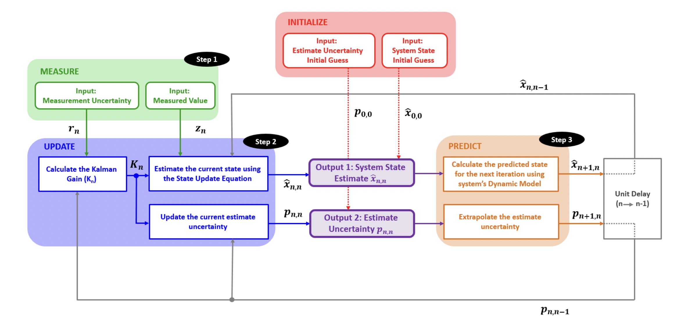
  • 算法流程：Initilize -> Loop(Measure -> Update -> Predict)

例5: 测一栋楼的高度

• 和例 1 测黄金的重量是一类问题，细节略
• 展示了 Kalman Filter 算法的工作流程，结论是测量误差和 Kalman Gain 都越来越小

完整的一维 Kalman Filter ——考虑 Process Noise

• 新的概念：
  • 之前假定系统的 Dynamic Model 没有误差，事实不是如此
  • Process Noise Variance: 反映 Dynamic Model 的误差，记为 $q$。
  • Covariance Extrapolation Equation 变为：$p_{n+1,n} = p_{n,n} + q_n$ (for constant dynamics)。

例6: 测量一盒液体的温度

• 温度可能由随机波动，System Dynamic 公式为 $x_n = T + w_n$
  • $T$ 是温度常量，$w_n$ 是温度波动，方差为 $q$。
• 此时温度真实值在波动，Kalman Filter 同样可以不断减小测量误差，计算过程略。

例7: 测量一盒正在加热的液体的温度

• 液体正在加热，同时温度波动的方差很小 $q = 0.0001$，但 Dynamic Model 仍假设液体问题不变
  • 出现了显著的 Lag Error, 这是由于 $q$ 很小导致了 $p$ 很小，使得 Kalman Gain 很小
  • 加上数学模型不正确，估计值不能很好的跟上测量值的变化

例8: 测量一盒正在加热的液体的温度 II

• 和上例唯一不同的地方在于，这次的 Process Noise 假设很大 $q=0.15$，但 Dynamic Model 仍假设液体温度不变
  • 在数学模型错误的情况下，没有出现 Lag Error, 估计值较为准确
  • 这是由于 $q$ 变大导致 $p$ 变大，进而 Kalman Gain 变大，估计值可以跟上测量值的变化
  • 换言之，将数学模型的错误考虑进来，增加了 $q$, 使估计结果变好
• 对比例 7 和例 8, 在数学模型均不对时，理论上此时有较大的 Process Noise, 因此 $q$ 更大者结果更好
• 理想的 Kalman Filter 应该具有接近真实情况的 Dynamic Model, 但现实应用中往往不成立，此时应该设置较大的 Process Noise 来充分考虑数学模型的误差。

---

Multidimensional Kalman Filter

Background

• 处理高维数据的测量，例如飞机运动的系统状态是一个 9 维向量：$[x,y,z,v_x,v_y,v_z,a_x,a_y,a_z]$。
• 需要用到概率统计的一些公式，例如概率勾股定理 $V(X) = E(X^2) - \mu_X^2$。

State Extrapolation Equation

• 通用形式：$\boldsymbol{\hat{x}{n+1,n} = F\hat{x}{n,n} + Gu_n + w_n}$。
  • $\boldsymbol{\hat{x}_{n+1,n}}$: 系统在 n+1 时刻的预测状态。
  • $\boldsymbol{\hat{x}_{n,n}}$: 系统在 n 时刻的估计状态。
  • $\boldsymbol{u_n}$: Control Variable 或 Input Variable, 可以被测量。
  • $\boldsymbol{w_n}$: Process Noise, 无法测量的干扰。
  • $\boldsymbol{F}$: State Transition Matrix.
  • $\boldsymbol{G}$: Control Matrix / Input Transition Matrix.

例9: Airplane - No Control Input

• 假设要追踪飞机的 9 维运动状态，没有 Control Input, 即 $\boldsymbol{u_n=0}$。

• 系统状态为 $\boldsymbol{\hat{x}_{n}} = [\hat{x}_n,\hat{y}_n,\hat{z}_n,\hat{\dot{x}}_n,\hat{\dot{y}}_n,\hat{\dot{z}}_n,\hat{\ddot{x}}_n,\hat{\ddot{y}}_n,\hat{\ddot{z}}_n]^T$。

• State Transition Matrix 为：

  • \[\boldsymbol{F} = \begin{bmatrix} & 1 & 0 & 0 & \Delta t & 0 & 0 & 0.5\Delta t^2 & 0 & 0 \\ & 0 & 1 & 0 & 0 & \Delta t & 0 & 0 & 0.5\Delta t^2 & 0 \\ & 0 & 0 & 1 & 0 & 0 & \Delta t & 0 & 0 & 0.5\Delta t^2 \\ & 0 & 0 & 0 & 1 & 0 & 0 & \Delta t & 0 & 0 \\ & 0 & 0 & 0 & 0 & 1 & 0 & 0 & \Delta t & 0 \\ & 0 & 0 & 0 & 0 & 0 & 1 & 0 & 0 & \Delta t \\ & 0 & 0 & 0 & 0 & 0 & 0 & 1 & 0 & 0 \\ & 0 & 0 & 0 & 0 & 0 & 0 & 0 & 1 & 0 \\ & 0 & 0 & 0 & 0 & 0 & 0 & 0 & 0 & 1 \\ \end{bmatrix}\]

• State Extrapolation Equation: $\boldsymbol{\hat{x}{n+1,n} = F\hat{x}{n,n}}$

例9: Airplane with Control Input

• 这次要追踪飞机的位移和速度 6 维运动状态，但飞机上有测量装置可以测量 3 维加速度。

• 系统状态 $\boldsymbol{\hat{x}{n}}=[\hat{x}_n,\hat{y}_n,\hat{z}_n,\hat{\dot{x}}_n,\hat{\dot{y}}_n,\hat{\dot{z}}_n]^T$, Control Input 为 $\boldsymbol{u_n} = [\hat{\ddot{x}}{n},\hat{\ddot{y}}{n},\hat{\ddot{z}}{n}]$。

• State Transition Matrix 为：

  • \[\boldsymbol{F} = \begin{bmatrix} & 1 & 0 & 0 & \Delta t & 0 & 0 \\ & 0 & 1 & 0 & 0 & \Delta t & 0 \\ & 0 & 0 & 1 & 0 & 0 & \Delta t \\ & 0 & 0 & 0 & 1 & 0 & 0 \\ & 0 & 0 & 0 & 0 & 1 & 0 \\ & 0 & 0 & 0 & 0 & 0 & 1 \\ \end{bmatrix}\]

• Control Matrix 为：

  • \[\boldsymbol{G} = \begin{bmatrix} & 0.5\Delta t^2 & 0 & 0 \\ & 0 & 0.5\Delta t^2 & 0 \\ & 0 & 0 & 0.5\Delta t^2 \\ & \Delta t & 0 & 0 \\ & 0 & \Delta t & 0 \\ & 0 & 0 & \Delta t \\ \end{bmatrix}\]

• State Extrapolation Equation 为 $\boldsymbol{\hat{x}{n+1,n} = F\hat{x}{n,n} + Gu_{n,n}}$。

• 注意这个问题和 IMU 不一样，IMU 坐标系和全局坐标系不统一，差一个转化步骤。

例10: 自由落体

• 系统状态是物体高度和速度，Control Input 是重力加速度常量 $g$。
• 公式很简单，略。

Modeling Linear Dynamics Systems

• 很有挑战性的一章，扩展到一般性的线性系统

  • 通用 State Extrapolation Equation: $\boldsymbol{\hat{x}{n+1,n} = F\hat{x}{n,n} + G\hat{u}_{n,n} + w_n}$。

  • 通用的 Dynamic Model:

    • \[\left\{ \begin{aligned} & \boldsymbol{\dot{x}(t) = Ax(t) + Bu(t)} \\ & \boldsymbol{y(t) = Cx(t) + Du(t)} \\ \end{aligned} \right.\]
    • where $\boldsymbol{x}$ is the state vector; $\boldsymbol{y}$ is the output vector; $\boldsymbol{A}$ is the system’s dynamics matrix; $\boldsymbol{B}$ is the input matrix; $\boldsymbol{C}$ is the output matrix; $\boldsymbol{D}$ is the feedthrough matrix.

  • 通过求解 Dynamic Model 确定 State Extrapolation Equation 中的 F 和 G。

例11: 匀速直线运动的通用 Dynamic Model

• 设系统的状态向量为 $\boldsymbol{x} = [p, v]^T$, 位移和速度；系统的输出为位移标量。

• 因为匀速直线运动，系统没有力的输入，则 $\boldsymbol{u(t)} = 0$。

• 则系统的通用 Dynamic Model 为：

  • \[\left\{ \begin{aligned} & \begin{bmatrix} \dot{p} \\ \dot{v} \\ \end{bmatrix} = \begin{bmatrix} 0 & 1 \\ 0 & 0 \\ \end{bmatrix} \begin{bmatrix} p \\ v \\ \end{bmatrix} + \boldsymbol{0} \\ & p = \begin{bmatrix} 1 & 0 \\ \end{bmatrix} \begin{bmatrix} p \\ v \end{bmatrix} + \boldsymbol{0} \end{aligned} \right.\]

处理高次微分方程的方法

• 将一个变量展开，用 n 个变量分别表示原来变量的不同次微分，则原 n 次微分方程可以写成 1 次微分方程组，转化为通用的矩阵形式，数学推导略。

例12: 匀加速直线运动

• 有外力作用在物体上，做匀加速运动。

  • 应用牛顿第二定律，微分方程的约束为 $m\ddot{p} = F$。

• 推导 Dynamic Model 方程组：

  • \[\left\{ \begin{aligned} & \begin{bmatrix} \dot{p} \\ \dot{v} \end{bmatrix} = \begin{bmatrix} 0 & 1 \\ 0 & 0 \\ \end{bmatrix} \begin{bmatrix} p \\ v \end{bmatrix} + \begin{bmatrix} 0 \\ \cfrac{1}{m} \end{bmatrix} F \\ & p = \begin{bmatrix} 1 & 0 \\ \end{bmatrix} \begin{bmatrix} p \\ v \end{bmatrix} + [0] \cfrac{F}{m} \end{aligned} \right.\]

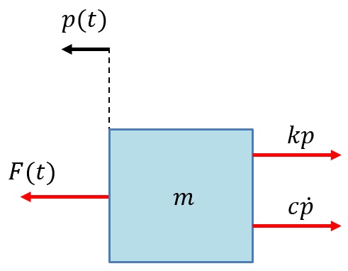
例13: 连接有弹簧和阻尼器的物块的运动

• 一个质量 $m$ 的物块受向左的外力 $F(t)$ 和向右的弹簧拉力和阻尼器阻力，受力分析图如下：
  • 

• 2 次微分方程：$F(t)-kp-c\dot{p} = m\ddot{p}$。

• 对应的微分方程组：

  • \[\left\{ \begin{aligned} & \begin{bmatrix} \dot{p} \\ \dot{v} \end{bmatrix} = \begin{bmatrix} 0 & 1 \\ -\cfrac{k}{m} & -\cfrac{c}{m} \end{bmatrix} \begin{bmatrix} p \\ v \end{bmatrix} + \begin{bmatrix} 0 \\ \cfrac{1}{m} \\ \end{bmatrix} F \\ & p = \begin{bmatrix} 1 & 0 \\ \end{bmatrix} \begin{bmatrix} p \\ v \\ \end{bmatrix} + [0] \cfrac{F}{m} \end{aligned} \right.\]

求解微分方程组

• 一维微分方程 $\dot{x} = kx$ 的解为 $x = x_0e^{k\Delta t}$。
• 推广到高维可得微分方程组 $\boldsymbol{\dot{x} = Ax}$ 的解为 $\boldsymbol{x_{n+1} = x_ne^{A\Delta t}}$
  • 其中 $\boldsymbol{e^X}$ 是矩阵指数幂，$e^{\boldsymbol{X}} = \sum_{k=0}^{\infin}\cfrac{1}{k!}\boldsymbol{X}^k$, 如果 $\boldsymbol{X}$ 是幂零矩阵，则泰勒展开只有有限项不为 0。
• 通过上面两个例子我们得到了通用矩阵形式的微分方程组，最终目的是求解方程组得到通用的 System Extrapolation Equation。

例11 continued: 匀速直线运动

• \[\begin{aligned} & \boldsymbol{\dot{x} = Ax \rightarrow x_{n+1} = e^{A\Delta t}x_n} \\ & \boldsymbol{A} = \begin{bmatrix} 0 & 1 \\ 0 & 0 \end{bmatrix} \\ & F = \boldsymbol{e^{A\Delta t} = \sum_{k=0}^{\infin}}\cfrac{1}{k}(A\Delta t)^k = I + A\Delta t = \begin{bmatrix} 1 & \Delta t \\ 0 & 1 \\ \end{bmatrix} \\ & \begin{bmatrix} x_{n+1} \\ \dot{x}_{n+1} \end{bmatrix} = \begin{bmatrix} 1 & \Delta t \\ 0 & 1 \\ \end{bmatrix} \begin{bmatrix} x_n \\ \dot{x}_{n} \\ \end{bmatrix} \end{aligned}\]

带有输入向量的系统

• $u(t) \ne 0$, 此时 Dynamic Model 为 $\boldsymbol{\dot{x}(t) = Ax(t) + Bu(t)}$。

• 直接给出微分方程组的解：

  • \[\begin{aligned} & \boldsymbol{x(t+\Delta t) = e^{A\Delta t}x(t) + \int_{0}^{\Delta t}e^{At}dtBu(t)} \\ & where: \boldsymbol{F = e^{A\Delta t}, G = \int_{0}^{\Delta t}e^{At}dtB} \\ \end{aligned}\]
  • 直接带入 System Extrapolation Equation 即可。

• 复杂的微分方程可以使用数值软件求解。

Covariance Extrapolation Equation

• 矩阵形式的通用公式：$\boldsymbol{P_{n+1,n} = FP_{n,n}F^T + Q}$
  • $\boldsymbol{P_{n,n}}$: 当前估计值的不确定性 - covariance matrix of the current state.
  • $\boldsymbol{P_{n+1,n}}$: 下一次预测的不确定性 - covariance metrix of the next state.
  • $\boldsymbol{F}$: state transition matrix, 和之前相同。
  • $\boldsymbol{Q}$: the process noise matrix.

没有模型误差的估计 The Estimate Uncertainty without the Process Noise

• 没有模型误差时 $\boldsymbol{Q} = 0$, 则 $\boldsymbol{P_{n+1,n} = FP_{n,n}F^T}$, 下面证明该公式。

• 根据定义，已知 $\boldsymbol{P_{n,n}=E((\hat{x}{n,n}-\mu{x_{n,n}})(\hat{x}{n,n}-\mu{x_{n,n}})^T)}$, $\boldsymbol{\hat{x}{n+1,n}=F\hat{x}{n,n}+G\hat{u}_{n,n}}$, 则有：

  • \[\begin{aligned} P_{n+1,n} & = E((\hat{x}_{n+1,n}-\mu_{x_{n+1,n}})(\hat{x}_{n+1,n}-\mu_{x_{n+1,n}})^T) \\ & = E((F\hat{x}_{n,n}+G\hat{u}_{n,n}-F\mu_{x_{n,n}}-G\hat{u}_{n,n})(F\hat{x}_{n,n}+G\hat{u}_{n,n}-F\mu_{x_{n,n}}-G\hat{u}_{n,n})^T) \\ & = E(F(\hat{x}_{n,n}-\mu_{x_{n,n}})(F(\hat{x}_{n,n}-\mu_{x_{n,n}}))^T) \\ & = FE((\hat{x}_{n,n}-\mu_{x_{n,n}})(\hat{x}_{n,n}-\mu_{x_{n,n}})^T)F^T \\ & = FP_{n,n}F^T \\ \end{aligned}\]

构造模型误差矩阵 Constructing the Process Noise Matrix Q

• Dynamic Model again: $\boldsymbol{\hat{x}{n+1,n}=F\hat{x}{n,n}+G\hat{u}_{n,n}+w_n}$.
• $\boldsymbol{w_n}$ 是 Process Noise, 一维误差（方差）为 $q$, 高维误差（协方差矩阵）为 $\boldsymbol{Q}$。
• 如果状态内各变量无关，则误差矩阵为对角阵。
• Process Noise 有两种误差模型：离散误差模型和连续误差模型。
  • 离散模型：假设误差在每个时刻不同，但在时刻间保持不变。
  • 连续模型：假设误差在不同时刻连续变化。

例12: 匀加速直线运动

• 模型假设加速度为 0, 但实际加速度有很小的波动，加速度误差为 $\sigma_a^2$。

• 系统状态为 $[x, v]$ 分别表示速度和位移，则矩阵 Q 如下：

  • \[\begin{aligned} Q & = \begin{bmatrix} V(x) & COV(x,v) \\ COV(x,v) & V(v) \\ \end{bmatrix} \\ V(x) & = E(x^2) - E(x)^2 = E((\cfrac{1}{2}a\Delta t^2)^2) - E(\cfrac{1}{2}a\Delta t^2)^2 = \cfrac{1}{4}\sigma_a^2\Delta t^4 \\ V(v) & = E(v^2) - E(v)^2 = E((a\Delta t)^2) - E(a\Delta t) = \sigma_a^2\Delta t^2 \\ COV(x,v) & = E(xv) - E(x)E(v) = E(\cfrac{1}{2}a^2\Delta t^3) - E(\cfrac{1}{2}a\Delta t^2)E(a\Delta t) = \cfrac{1}{2}\sigma_a^2\Delta t^3 \\ \end{aligned}\]

Measurement Equation

• 是一个辅助公式，不属于五大公式之一，矩阵形式通用公式：$\boldsymbol{z_n = Hx_n + v_n}$。
  • $\boldsymbol{z_n}$: the measurement vector 测量值。
  • $\boldsymbol{x_n}$: the true system state(hidden) 系统隐藏的真实状态。
  • $\boldsymbol{v_n}$: the random noise vector 随机误差，方差为 $\boldsymbol{r_n}$。
  • $\boldsymbol{H}$: the observation matrix 观测矩阵。

观测矩阵 The Observation Matrix H

• Intuition: 从测量值不一定能直接得到系统状态，中间需要一个矩阵做变换，这个矩阵就是 H。
  • 例如，系统状态是温度，但由电子温度计得到的测量值是电流。
  • 例如，系统状态是位移、速度和姿态角，由 IMU 得到的是加速度和角速度。
• 观测矩阵 H 的不同情况：
  • Scaling: 系统状态到测量值有一个倍数，利于光反射通过时间测距离。
  • State Selection: 只有一部分系统状态可以测量，比如加速度。
  • Combination of States: 系统状态但变量不可测量，但变量的组合可以测量。

Interim Summary

Prediction Equations

• State Extrapolation Equation: $\boldsymbol{\hat{x}{n+1,n}=F\hat{x}{n,n}+Gu_n+w_n}$.
• Covariance Extrapolation Equation: $\boldsymbol{P_{n+1,n}=FP_{n,n}F^T+Q}$.

Auciliary Equations

• Measurement Equation: $\boldsymbol{z_n=Hx_n+v_n}$.
• Covariance Equations: all covariance equations are covariance matrices in the form of $\boldsymbol{E(ee^T})$.
  • Measurement Uncertainty: $\boldsymbol{R_n=E(v_nv_n^T)}$.
  • Process Noise Unvertainty: $\boldsymbol{Q_n=E(w_nw_n^T)}$.
  • Estimation Uncertainty: $\boldsymbol{P_{n,n}=E(e_ne_n^T)=E((x_n-\hat{x}{n,n})(x_n-\hat{x}{n,n})^T)}$.

State Update Equation

• 矩阵形式通用公式：$\boldsymbol{\hat{x}{n,n}=\hat{x}{n,n-1}+K_n(z_n-H\hat{x}_{n,n-1})}$。
  • $\boldsymbol{\hat{x}_{n,n}}$: 时刻 n 的状态估计值。
  • $\boldsymbol{\hat{x}_{n,n-1}}$: 时刻 n-1 时对时刻 n 的状态预测值。
  • $\boldsymbol{K_n}$: the Kalman Gain.
  • $\boldsymbol{z_n}$: 测量值 the measurement.
  • $\boldsymbol{H}$: 观测矩阵 the observation matrix.
• 注意公式中矩阵的维度，如果 $\boldsymbol{x,z}$ 分别为 $m,n$ 维，则 $\boldsymbol{K}$ 是 $m\times n$, $H$ 是 $n\times m$。

Covariance Update Equation

• 矩阵形式通用公式：$\boldsymbol{P_{n,n}=(I-K_nH)P_{n,n-1}(I-K_nH)^T+K_nR_nK_n^T}$。
  • $\boldsymbol{P_{n,n}}$: 时刻 n 的估计值不确定度。
  • $\boldsymbol{P_{n,n-1}}$: 时刻 n-1 预测的时刻 n 的不确定度。
  • $\boldsymbol{K_n}$：the Kalman Gain.
  • $\boldsymbol{H}$: 观测矩阵 the observation matrix.
  • $\boldsymbol{R_n}$: 测量值不确定度 the Measurement Uncertainty.
  • $\boldsymbol{I}$: 单位矩阵。

公式推导过程

• 使用如下公式：

  • $(1)\ \boldsymbol{\hat{x}{n,n}=\hat{x}{n,n-1}+K_n(z_n-\hat{x}_{n,n-1})}$.
  • $(2)\ \boldsymbol{z_n=Hx_n+v_n}.$
  • $(3)\ \boldsymbol{P_{n,n}=E((x_n-\hat{x}{n,n})(x_n-\hat{x}{n,n})^T)}.$
  • $(4)\ \boldsymbol{E(v_nv_n^T)}$.

• 推导过程：

  • \[\begin{aligned} P_{n,n} & = E((x_n-\hat{x}_{n,n})(x_n-\hat{x}_{n,n})^T)\ (1) \\ & = E((x_n-\hat{x}_{n,n-1}-K_n(z_n-H\hat{x}_{n,n-1}))(\sim)^T)\ (2) \\ & = E((x_n-\hat{x}_{n,n-1}-K_n(Hx_n+v_n-H\hat{x}_{n,n-1}))(\sim)^T) \\ & = E(((I-K_nH)(x_n-\hat{x}_{n,n-1})-K_nv_n)(\sim)^T) \\ & = E((I-K_nH)(x_n-\hat{x}_{n,n-1}(x_n-\hat{x}_{n,n-1})^T(I-K_nH)^T)) \\ & - E(K_nv_n(x_n-\hat{x}_{n,n-1})^T(I-K_nH)^T)\ (v_n\ is\ not\ correalated\ with\ (x_n-\hat{x}_{n,n-1}))\\ & - E((I-K_nH)(x_n-\hat{x}_{n,n-1})v_n^TK_N^T)\ (the\ same) \\ & + E(K_nv_nv_n^TK_n^T)\ (3,4) \\ & = (I-K_nH)P_{n,n-1}(I-K_nH)^T + K_nR_nK_n^T \end{aligned}\]

The Kalman Gain

• 矩阵形式通用公式：$\boldsymbol{K_n=P_{n,n-1}H^T(HP_{n,n-1}H^T+R_n)^{-1}}$。
  • 符号含义同上。

公式推导过程

• 基于 Covariance Update Equation, 选择合适的 $\boldsymbol{K_n}$ 使得 $\boldsymbol{P_{n,n}}$ 最小，本质是一个最优化问题。
• 需要用到矩阵微分，过程比较复杂，见推导过程，略。

Simplified Covariance Update Equation

• 简化的公式形式：$\boldsymbol{P_{n,n}=(I-K_nH)P_{n,n-1}}$。

公式推导过程

• 将 Covariance Update Equation 展开，然后代入上面推导出的 Kalman Gain Equation, 就会得到这个简洁的公式。
• 注意：$\boldsymbol{(I-K_nH)}$ 因数值数值不稳定，慎用。

Summary

• 现在总结 Kalman Filter 中用到的所有公式。

Predict Equations

• State Extrapolation Equation: $\boldsymbol{\hat{x}{n+1,n}=F\hat{x}{n,n}+Gu_n}$.
• Covariance Extrapolation Equation: $\boldsymbol{P_{n+1,n}=FP_{n,n}F^T+Q}$.

Update Equations

• State Update Equation: $\boldsymbol{\hat{x}{n,n}=\hat{x}{n,n-1}+K_n(z_n-H\hat{x}_{n,n-1})}$.
• Covariance Update Equation: $\boldsymbol{P_{n,n}=(I-K_nH)P_{n,n-1}(I-K_nH)^T}+K_nR_nK_n^T$.
• Kalman Gain Equation: $\boldsymbol{K_n=P_{n,n-1}H^T(HP_{n,n-1}H^T+R_n)^{-1}}$.

Auxiliary Equations

• Measurement Equation: $\boldsymbol{z_n=Hx_n+v_n}$.
• Measurement Uncertainty: $\boldsymbol{R_n=E(v_nv_n^T)}$.
• Process Noise Uncertainty: $\boldsymbol{Q_n=E(w_nw_n^T)}$.
• Estimate Uncertainty: $\boldsymbol{P_{n,n}=E(e_ne_n^T)=E((x_n-\hat{x}{n,n})(x_n-\hat{x}{n,n})^T)}$.

---

• Previous
  Hello World, to github.io
• Next
  Allan Variance 学习笔记

---